Statistical analysis made easy in Python with SciPy and pandas DataFrames
I finally got around to finishing up this tutorial on how to use pandas DataFrames and SciPy together to handle any and all of your statistical needs in Python. This is basically an amalgamation of my two previous blog posts on pandas and SciPy.
This is all coded up in an IPython Notebook, so if you want to try things out for yourself, everything you need is available on github: https://github.com/briandconnelly/BEACONToolkit/tree/master/analysis/scripts
Statistical Analysis in Python
In this section, we introduce a few useful methods for analyzing your data in Python. Namely, we cover how to compute the mean, variance, and standard error of a data set. For more advanced statistical analysis, we cover how to perform a Mann-Whitney-Wilcoxon (MWW) RankSum test, how to perform an Analysis of variance (ANOVA) between multiple data sets, and how to compute bootstrapped 95% confidence intervals for non-normally distributed data sets.
Python’s SciPy Module
The majority of data analysis in Python can be performed with the SciPy module. SciPy provides a plethora of statistical functions and tests that will handle the majority of your analytical needs. If we don’t cover a statistical function or test that you require for your research, SciPy’s full statistical library is described in detail at: http://docs.scipy.org/doc/scipy/reference/tutorial/stats.html
Python’s pandas Module
The pandas module provides powerful, efficient, R-like DataFrame objects capable of calculating statistics en masse on the entire DataFrame. DataFrames are useful for when you need to compute statistics over multiple replicate runs.
For the purposes of this tutorial, we will use Luis Zaman’s digital parasite data set:
from pandas import * # must specify that blank space " " is NaN experimentDF = read_csv("parasite_data.csv", na_values=[" "]) print experimentDF [class 'pandas.core.frame.DataFrame'] Int64Index: 350 entries, 0 to 349 Data columns: Virulence 300 non-null values Replicate 350 non-null values ShannonDiversity 350 non-null values dtypes: float64(2), int64(1)
Accessing data in pandas DataFrames
You can directly access any column and row by indexing the DataFrame.
# show all entries in the Virulence column print experimentDF["Virulence"] 0 0.5 1 0.5 2 0.5 3 0.5 4 0.5 ... 346 NaN 347 NaN 348 NaN 349 NaN Name: Virulence, Length: 350
# show the 12th row in the ShannonDiversity column print experimentDF["ShannonDiversity"][12] 1.58981
You can also access all of the values in a column meeting a certain criteria.
# show all entries in the ShannonDiversity column > 2.0 print experimentDF[experimentDF["ShannonDiversity"] > 2.0] Virulence Replicate ShannonDiversity 8 0.5 9 2.04768 89 0.6 40 2.01066 92 0.6 43 2.90081 96 0.6 47 2.02915 ... 235 0.9 36 2.19565 237 0.9 38 2.16535 243 0.9 44 2.17578 251 1.0 2 2.16044
Blank/omitted data (NA or NaN) in pandas DataFrames
Blank/omitted data is a piece of cake to handle in pandas. Here’s an example data set with NA/NaN values.
import numpy as np print experimentDF[np.isnan(experimentDF["Virulence"])] Virulence Replicate ShannonDiversity 300 NaN 1 0.000000 301 NaN 2 0.000000 302 NaN 3 0.833645 303 NaN 4 0.000000 ... 346 NaN 47 0.000000 347 NaN 48 0.444463 348 NaN 49 0.383512 349 NaN 50 0.511329
DataFrame methods automatically ignore NA/NaN values.
print "Mean virulence across all treatments:", experimentDF["Virulence"].mean() Mean virulence across all treatments: 0.75
However, not all methods in Python are guaranteed to handle NA/NaN values properly.
from scipy import stats print "Mean virulence across all treatments:", stats.sem(experimentDF["Virulence"]) Mean virulence across all treatments: nan
Thus, it behooves you to take care of the NA/NaN values before performing your analysis. You can either:
(1) filter out all of the entries with NA/NaN
# NOTE: this drops the entire row if any of its entries are NA/NaN! print experimentDF.dropna() [class 'pandas.core.frame.DataFrame'] Int64Index: 300 entries, 0 to 299 Data columns: Virulence 300 non-null values Replicate 300 non-null values ShannonDiversity 300 non-null values dtypes: float64(2), int64(1)
If you only care about NA/NaN values in a specific column, you can specify the column name first.
print experimentDF["Virulence"].dropna() 0 0.5 1 0.5 2 0.5 3 0.5 ... 296 1 297 1 298 1 299 1 Name: Virulence, Length: 300
(2) replace all of the NA/NaN entries with a valid value
print experimentDF.fillna(0.0)["Virulence"] 0 0.5 1 0.5 2 0.5 3 0.5 4 0.5 ... 346 0 347 0 348 0 349 0 Name: Virulence, Length: 350
Take care when deciding what to do with NA/NaN entries. It can have a significant impact on your results!
print ("Mean virulence across all treatments w/ dropped NaN:", experimentDF["Virulence"].dropna().mean()) print ("Mean virulence across all treatments w/ filled NaN:", experimentDF.fillna(0.0)["Virulence"].mean()) Mean virulence across all treatments w/ dropped NaN: 0.75 Mean virulence across all treatments w/ filled NaN: 0.642857142857
Mean of a data set
The mean performance of an experiment gives a good idea of how the experiment will turn out on average under a given treatment.
Conveniently, DataFrames have all kinds of built-in functions to perform standard operations on them en masse: `add()`, `sub()`, `mul()`, `div()`, `mean()`, `std()`, etc. The full list is located at: http://pandas.pydata.org/pandas-docs/stable/api.html#computations-descriptive-stats
Thus, computing the mean of a DataFrame only takes one line of code:
from pandas import * print ("Mean Shannon Diversity w/ 0.8 Parasite Virulence =", experimentDF[experimentDF["Virulence"] == 0.8]["ShannonDiversity"].mean()) Mean Shannon Diversity w/ 0.8 Parasite Virulence = 1.2691338188
Variance in a data set
The variance in the performance provides a measurement of how consistent the results of an experiment are. The lower the variance, the more consistent the results are, and vice versa.
Computing the variance is also built in to pandas DataFrames:
from pandas import * print ("Variance in Shannon Diversity w/ 0.8 Parasite Virulence =", experimentDF[experimentDF["Virulence"] == 0.8]["ShannonDiversity"].var()) Variance in Shannon Diversity w/ 0.8 Parasite Virulence = 0.611038433313
Standard Error of the Mean (SEM)
Combined with the mean, the SEM enables you to establish a range around a mean that the majority of any future replicate experiments will most likely fall within.
pandas DataFrames don’t have methods like SEM built in, but since DataFrame rows/columns are treated as lists, you can use any NumPy/SciPy method you like on them.
from pandas import * from scipy import stats print ("SEM of Shannon Diversity w/ 0.8 Parasite Virulence =", stats.sem(experimentDF[experimentDF["Virulence"] == 0.8]["ShannonDiversity"])) SEM of Shannon Diversity w/ 0.8 Parasite Virulence = 0.110547585529
A single SEM will usually envelop 68% of the possible replicate means and two SEMs envelop 95% of the possible replicate means. Two SEMs are called the “estimated 95% confidence interval.” The confidence interval is estimated because the exact width depend on how many replicates you have; this approximation is good when you have more than 20 replicates.
Mann-Whitney-Wilcoxon (MWW) RankSum test
The MWW RankSum test is a useful test to determine if two distributions are significantly different or not. Unlike the t-test, the RankSum test does not assume that the data are normally distributed, potentially providing a more accurate assessment of the data sets.
As an example, let’s say we want to determine if the results of the two following treatments significantly differ or not:
# select two treatment data sets from the parasite data treatment1 = experimentDF[experimentDF["Virulence"] == 0.5]["ShannonDiversity"] treatment2 = experimentDF[experimentDF["Virulence"] == 0.8]["ShannonDiversity"] print "Data set 1:\n", treatment1 print "Data set 2:\n", treatment2 Data set 1: 0 0.059262 1 1.093600 2 1.139390 3 0.547651 ... 45 1.937930 46 1.284150 47 1.651680 48 0.000000 49 0.000000 Name: ShannonDiversity Data set 2: 150 1.433800 151 2.079700 152 0.892139 153 2.384740 ... 196 2.077180 197 1.566410 198 0.000000 199 1.990900 Name: ShannonDiversity
A RankSum test will provide a P value indicating whether or not the two distributions are the same.
from scipy import stats z_stat, p_val = stats.ranksums(treatment1, treatment2) print "MWW RankSum P for treatments 1 and 2 =", p_val MWW RankSum P for treatments 1 and 2 = 0.000983355902735
If P <= 0.05, we are highly confident that the distributions significantly differ, and can claim that the treatments had a significant impact on the measured value. If the treatments do not significantly differ, we could expect a result such as the following:
treatment3 = experimentDF[experimentDF["Virulence"] == 0.8]["ShannonDiversity"] treatment4 = experimentDF[experimentDF["Virulence"] == 0.9]["ShannonDiversity"] print "Data set 3:\n", treatment3 print "Data set 4:\n", treatment4 Data set 3: 150 1.433800 151 2.079700 152 0.892139 153 2.384740 ... 196 2.077180 197 1.566410 198 0.000000 199 1.990900 Name: ShannonDiversity Data set 4: 200 1.036930 201 0.938018 202 0.995956 203 1.006970 ... 246 1.564330 247 1.870380 248 1.262280 249 0.000000 Name: ShannonDiversity
# compute RankSum P value z_stat, p_val = stats.ranksums(treatment3, treatment4) print "MWW RankSum P for treatments 3 and 4 =", p_val MWW RankSum P for treatments 3 and 4 = 0.994499571124
With P > 0.05, we must say that the distributions do not significantly differ. Thus changing the parasite virulence between 0.8 and 0.9 does not result in a significant change in Shannon Diversity.
One-way analysis of variance (ANOVA)
If you need to compare more than two data sets at a time, an ANOVA is your best bet. For example, we have the results from three experiments with overlapping 95% confidence intervals, and we want to confirm that the results for all three experiments are not significantly different.
treatment1 = experimentDF[experimentDF["Virulence"] == 0.7]["ShannonDiversity"] treatment2 = experimentDF[experimentDF["Virulence"] == 0.8]["ShannonDiversity"] treatment3 = experimentDF[experimentDF["Virulence"] == 0.9]["ShannonDiversity"] print "Data set 1:\n", treatment1 print "Data set 2:\n", treatment2 print "Data set 3:\n", treatment3 Data set 1: 100 1.595440 101 1.419730 102 0.000000 103 0.000000 ... 146 0.000000 147 1.139100 148 2.383260 149 0.056819 Name: ShannonDiversity Data set 2: 150 1.433800 151 2.079700 152 0.892139 153 2.384740 ... 196 2.077180 197 1.566410 198 0.000000 199 1.990900 Name: ShannonDiversity Data set 3: 200 1.036930 201 0.938018 202 0.995956 203 1.006970 ... 246 1.564330 247 1.870380 248 1.262280 249 0.000000 Name: ShannonDiversity
# compute one-way ANOVA P value from scipy import stats f_val, p_val = stats.f_oneway(treatment1, treatment2, treatment3) print "One-way ANOVA P =", p_val One-way ANOVA P = 0.381509481874
If P > 0.05, we can claim with high confidence that the means of the results of all three experiments are not significantly different.
Bootstrapped 95% confidence intervals
Oftentimes in wet lab research, it’s difficult to perform the 20 replicate runs recommended for computing reliable confidence intervals with SEM.
In this case, bootstrapping the confidence intervals is a much more accurate method of determining the 95% confidence interval around your experiment’s mean performance.
Unfortunately, SciPy doesn’t have bootstrapping built into its standard library yet. However, there is already a scikit out there for bootstrapping. Enter the following command to install it:
sudo easy_install scikits.bootstrap
Bootstrapping 95% confidence intervals around the mean with this function is simple:
# subset a list of 10 data points treatment1 = experimentDF[experimentDF["Virulence"] == 0.8]["ShannonDiversity"][:10] print "Small data set:\n", treatment1 Small data set: 150 1.433800 151 2.079700 152 0.892139 153 2.384740 154 0.006980 155 1.971760 156 0.000000 157 1.428470 158 1.715950 159 0.000000 Name: ShannonDiversity
import scipy import scikits.bootstrap as bootstrap # compute 95% confidence intervals around the mean CIs = bootstrap.ci(data=treatment1, statfunction=scipy.mean) print "Bootstrapped 95% confidence intervals\nLow:", CIs[0], "\nHigh:", CIs[1] Bootstrapped 95% confidence intervals Low: 0.659028048 High: 1.722468024
Note that you can change the range of the confidence interval by setting the alpha:
# 80% confidence interval CIs = bootstrap.ci(treatment1, scipy.mean, alpha=0.2) print "Bootstrapped 80% confidence interval\nLow:", CIs[0], "\nHigh:", CIs[1] Bootstrapped 80% confidence interval Low: 0.827291024 High: 1.5420059
And also modify the size of the bootstrapped sample pool that the confidence intervals are taken from:
# bootstrap 20,000 samples instead of only 10,000 CIs = bootstrap.ci(treatment1, scipy.mean, n_samples=20000) print ("Bootstrapped 95% confidence interval w/ 20,000 samples\nLow:", CIs[0], "\nHigh:", CIs[1]) Bootstrapped 95% confidence interval w/ 20,000 samples Low: 0.644756972 High: 1.7071459
Generally, bootstrapped 95% confidence intervals provide more accurate confidence intervals than 95% confidence intervals estimated from the SEM.
Nice post. You may be interested in statsmodels. We take advantage of numpy, scipy, and pandas to provide statistical modeling. Here’s a linear model / ANOVA example
http://web.archive.org/web/20161011044754/http://statsmodels.sourceforge.net:80/devel/examples/generated/example_interactions.html
Perfect. This library may round off the final gap in Python stats that I’ve been looking to fill. Thanks so much for sharing it!
P.S. Any interest in merging a CI bootstrapping function into statsmodels? https://bitbucket.org/cevans/bootstrap
The author will release it fully under a BSD license soon.
Plenty of interest. Thanks for the pointer. We have some (parallel) bootstrapping right now in a few models, but nothing systematic yet. Long on the todo list. I filed an issue.
https://github.com/statsmodels/statsmodels/issues/420
Nice post. FYI, more bootstrap routines at
http://gcalmettes.github.com/bootstrap-tools/ (BSD license). Feel free to use it!
Nice library. Care to join the effort in getting bootstrapping merged into scipy.stats/statsmodels? 🙂
I’ve never actually seen sampling without replacement used for bootstrap samples. Unless I’m very mistaken, bootstrapping *requires* sampling with replacement, and Efron & Tibshirani doesn’t mention sampling without replacement; without replacement, each bootstrap sample will have the same value for the statistic. Indeed, your code seems to indicate that this is the case: try bootci(np.random.randn(100),mean,replacement=False) for example.
Is there some situation where sampling without replacement would work?
On the other hand, your code is much faster than mine for mean as the statistic, as you make a single call to the statistic function whereas I make n_sample calls to support functions that can’t apply themselves along an axis. I’m not sure which is the better way.
@Constantine thank you for getting in touch! Regarding your questions:
1) Indeed, Efron’s nonparametric bootstrap (1979) is the procedure of resampling with replacement from the original sample at the same sample size. However, Politis and Romano (1994) have also described resampling without replacement from the original sample at smaller size than the original sample size. In this case, subsampling bootstrap takes samples without replacement of size b from the original sample of size n, generally with b ≪ n. However, this is different enough from Efron’s idea that in their book (Politis, Romano, and Wolf, 1999) they don’t call it “bootstrap” but just plain “sub-sampling”.
2) The resampling without replacement can also be used when comparing two datasets (let’s say of size a and b respectively), for example, when you want to know if the difference between the mean of two datasets has been observed by chance. In this case, you can “pool” the two datasets into a big box (where all the data of the two datasets are merged) and then draw 10000 pseudo pair of samples (of size a and b) and see where the original calculated difference ranks in those dataset (see the bootpv function). This is like a pure. Of course, this procedure can also be done with replacement, but that is why I have a “Replacement=True/False” argument. If you are interested in the difference between with and without replacement for comparing two samples, see http://www.public.iastate.edu/~wrstephe/Resampling_Final.pdf for example.
3) yes, my code requires a function that can be apply on an axis, which can be a problem if someone has to use a custom function. I guess that this can be overcome by introducing a “try-except”-like statement in the code, and using the other method if an error occurs.
It’s worth noting that the scikits-bootstrap code you use can actually be very easily installed with pip. Just use
pip install -e git+http://github.org/cgevans/scikits-bootstrap.git#egg=Package
Then you can import scikits.bootstrap as bootstrap, or something similar.
Nicely done. Thanks again for reworking your bootstrapping function into a scikit, Constantine. 🙂
Thanks for your post!
When trying to run the bootstrap code, I found out the right parameter’s name is statfunction, not statfun and mentioned in the post.
Ah, that’s right, thanks! Guess that changed in the latest version of the bootstrapping code.
Hi Randall – I didn’t find method isnan in pandas. Instead I had to make this substitution:
from
experimentDF[isnan(experimentDF[“Virulence”])]
to:
import numpy as np
experimentDF[np.isnan(experimentDF[“Virulence”])]
I’m using pandas 0.9.0 (the latest as of this date).
Also parasite_data.csv has become perhaps harder to find. I found it buried in this project:
https://github.com/briandconnelly/BEACONToolkit
That’s strange about isnan. It was working in my version. 🙂 Nonetheless, I’ve updated the tutorial to correct that issue.
Here is a direct link to the directory parasite_data.csv is located in: https://github.com/briandconnelly/BEACONToolkit/tree/master/analysis/scripts/data-analysis-python
Thanks for pointing these out!
just a quick question: how do you make import work? the module’s name has a dot in it, ‘import scikit.bootstrap as bootsrap’ doesn’t work for me
If you’ve already installed scikit.bootstrap, check their docs to see if they changed the name of the module. They may have changed the scikit.bootstrap name since I wrote this post up.
I’ve just installed it, it’s still called scikits.bootstrap.. kinda weird, because import simply doesn’t work. I have to go like this:
>>> import imp
>>> bootstrap = imp.load_source(‘scikits.bootstrap’, ‘/home/me/scb/src/package/scikits/bootstrap/bootstrap.py’)
>>> bootstrap.ci
Maybe I should just head on directly to the github page..
I think so. I’ve never seen this before. Sorry!
Thanks for the post, man. It saves me some time coding stats in Python. I actually came across your page when working on a project in the same field of evolutionary robotics with Jeff Clune (probably you know him..) .. 🙂
Peace,
Anh
Would you know any packages which support post hoc tests for anova?
Check out statsmodels and see if they have it there. If not, you can always use Rmagic to run the specific test in R, then pass the result back to Python.
Great post! I try to implement bootstrap with grouped data (2d-array: x and weigths) but i don’t know how to do that. Have you any idea?
“If P > 0.05, we can claim with high confidence that the means of the results of all three experiments are not significantly different.”
I’m not sure exactly what you mean by this, but I think it is misleading.
If by “significantly different” you refer to statistical significance, then there is no claim–this is just a fact assuming you have set p=0.5 to be the significance threshold. If, on the other hand, you refer to colloquial significance, i.e. whether there is actually a meaningful difference between the two groups, then this claim would amount to “proving the null hypothesis”, which is something that you cannot do with a statistical test.
Great and practical article! and Check the course out from the link below.
http://www.thedevmasters.com/
First thank you for the post. Very useful and clear.
I have a related question. I have three means and the p-values showing that they are not the same. (0.002, 0.003 and 0.54) And it is clear that the first two very low values are not the same the last one is just over of the p<0.05 standard value. I would like to say I am XX% confident that they are not the same. Not just here is the mean and the 95% confidence interval around it is x and y. Is there a way to do this?
Thank you,
Noah